Project 3-1: Ray Tracing Part 1

Overview

In this project, I implemented the core routines of a physically-based renderer using a path-tracing algorithm. I developed algorithms for detecting ray-scene intersections. I built acceleration structures (BVHs) to speed up the CPU rendering time for large images, and I also physically simulated images based lighting and materials. Specifically, I deployed various illumination methods to achieve the final rendering results. To simulate the direct lighting effects, I used a combination of uniform hemisphere illumination and lighting sampling illumination. To simulate the bouncing of lights (or indirect lights), I used recursion with random termination depths like Russian roulette. I also added statistical analysis for early-stopping to reduce the need to sample locations unnecessarily if they are already rendered pretty well, as an additional way to accelerate my ray-tracing algorithms.

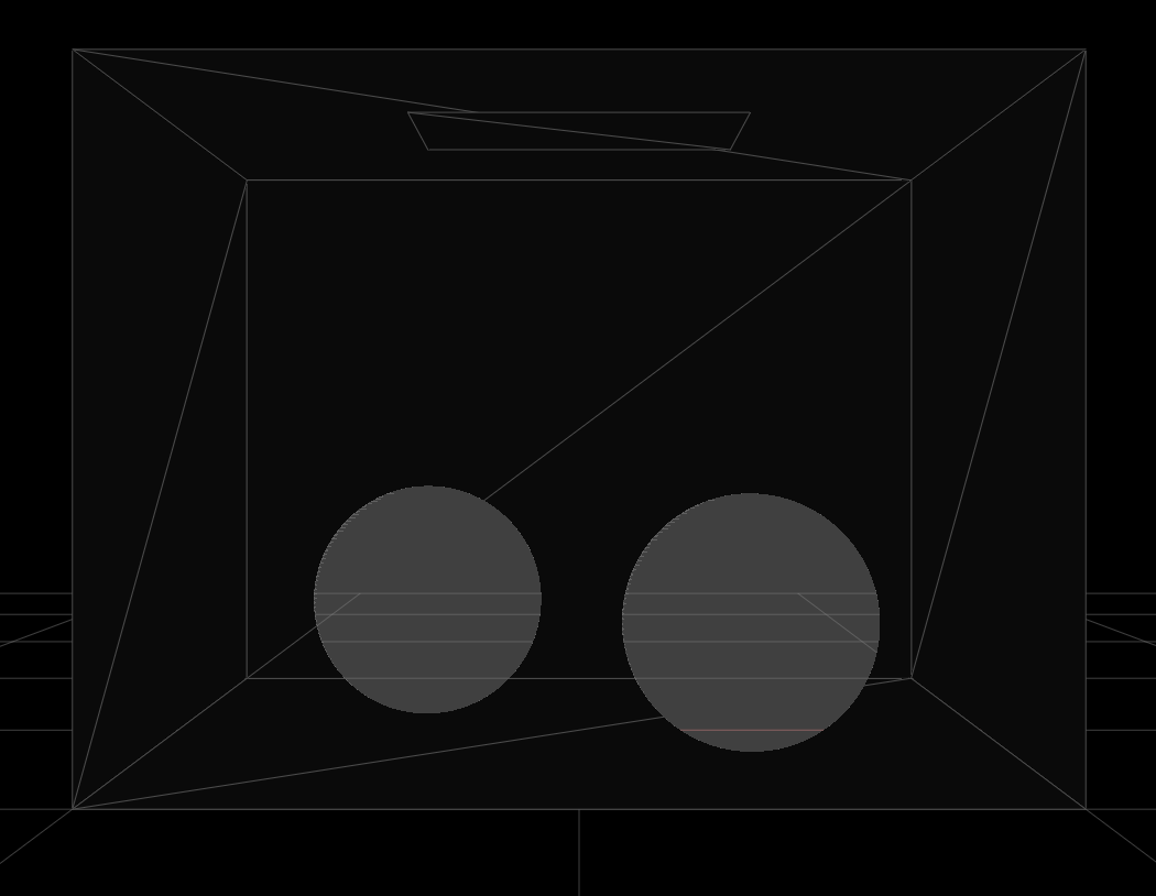
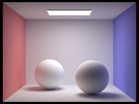
It's pretty amazing to see how we can generate relativistic images by simulating the physics of light and interactions in the physical real world. For example, as we can see below, we are able to generate a relativistic image of diffused material spheres in a box (on the right) based on physical ray-tracing on the model file (on the left). It's pretty astonishing.

Part 1: Ray Generation and Scene Intersection

For Ray tracing, we use a pinhole camera model. We shot virtual "eye rays" (or "camera rays" if shotting from a camera) and observe their intersections (reflections, intersections, refractions, etc.) with the physical world in order to assist us in rendering the images. Below is a visual description of what the pinhole camera model is:

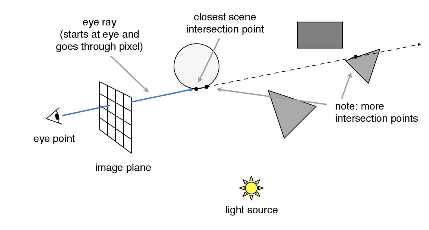
To generate a ray pointing from camera to a specfic point (x, y), we first notice that the camera has its own coordinate system, where the camera is positioned at the origin of the camera space, looking along the −z axis and having the +y axis as image space "up". Thus, the origin of our ray will simply be the world coordinates of the camera position, which is also the origin in the camera space. We can get the direction of the ray pointing to the point by finding the unit vector pointing from the camera to that point (x, y). Since we are given the horizontal field of view and vertical field of view angles of the camera, we can get the local coordinate of (x, y) in camera space by mapping (0,0) to bottom left (Vector3D(-tan(radians(hFov)*.5), -tan(radians(vFov)*.5),-1)) and (1,1) to top right (Vector3D( tan(radians(hFov)*.5), tan(radians(vFov)*.5),-1)) in the sensor. Then, we convert the directional vector to the normal vector in the world space, and then the origin and the direction forms the camera ray that we generated.

To test if the ray intersects with a triangle, we use the Moller Trumbore Algorithm below, which gives us the intersection point of an ray to a triangle defined by the three points P0, P1, and P2, if there is any valid intersection. It also gives us the barycentric coordinates that we can use to derive the normal vector of the intersection point.

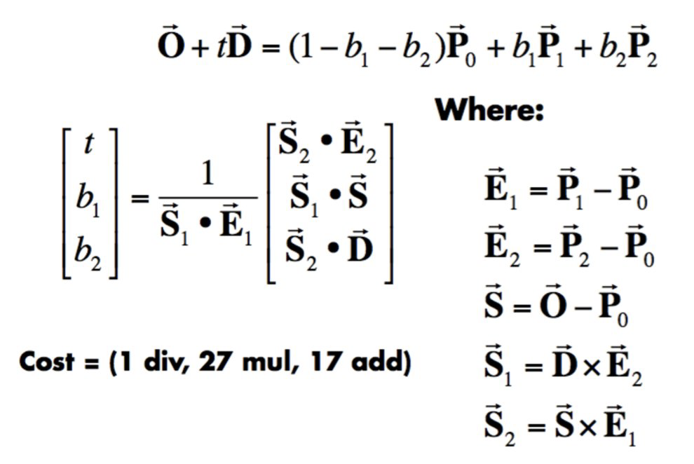
In a high level, what this algorithm is doing is that: from the perspective barycentric coordinates, the intersection point can always be interpreted as a linear combination among the three vertices, regardless of the coordinate system. At the same time, the intersection point can be parametrized by the origin of the ray, the direction of the ray, and the distance it traveled. Thus we can set up the equation at the to. Then, by moving parameters around, we can solve this system of equation for the distance traveled by the ray from the origin in the direction of its directional vector: t in a matrix form as described below in the algorithm. The value of b1 and b2 can also be derived from the equation by algebraic manipulations. If the distance traveled t is within the range of the ray segment (the start as r.min_t and the end as r.ax_t), we know it's a valid intersection. Otherwise, it's not.

To test the intersection against the sphere, we use a similar approach where we can solve the intersection points of an ray to a sphere in a closed quadratic form as below:

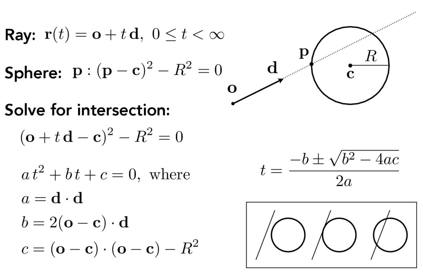
In a high level, I first calculate the delta b^2-4ac. If it's negative, the quadratic equation does not have a solution, so we don't have an intersection. If the value is zero, we have one intersection. If it's positive, we have two intersections. Once we solve for t, we then check, the same as what we did for the triangle case, if the distance traveled t is within the range of the ray segment (the start as r.min_t and the end as r.ax_t). If t1 (the smaller of the two t values) is in the range, it's the closet intersection we are looking for. If t1 is out of range but t2 is in the range, then t2 is our first intersection. Otherwise, there's still no intersections.

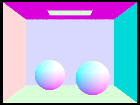
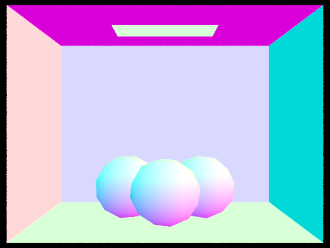
Below are some examples of rendered small .dae files:

Part 2: Bounding Volume Hierarchy

To accelerate the rendering pipeline, we used a technique called Bounding Volume Hierarchy (BVH), where we partition objects spatially into different bounding boxes. We test the existence of an intersection against each bounding box first, before we test intersections on each object. In this way, if a ray misses the bounding box, we don't have to test any of the objects inside, thus speeding up the process.

First, we will construct our BVH and spatially partition the objects into different bounding boxes, all stored in a tree-like structure as depicted below:

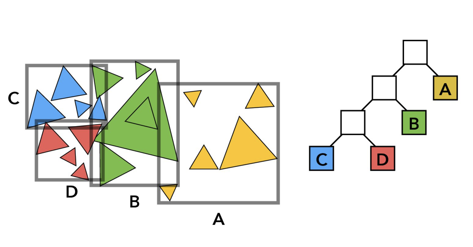
My BVH construct algorithm works as follows.

• Loop through all the objects (or primitives) needed for partition and create a tight bounding box that contains all the primitives.
• If the number of primitives left is no more than the max number of primitives we store for each leaf node, we contain all the primitives in a leaf node and terminate the algorithm, as we have met our termination criteria.
• Otherwise, we pick the axis of the current bounding box (which contains all current primitives from first step) that has the biggest extent (or length of axis). We split at the midpoint of this axis.
• We loop through every primitive. If the centroid of the primitive is on the left side of the split midpoint, we assign it to the left cluster. Otherwise, we put it in the right cluster.
• Then, we recursively repeat the above instructions on these clusters to construct BVHs for these sub-clusters, until all primitives are split and assigned to a leaf node.
• However, there are few edge cases we will deal with. The heuristic I chose here is the midpoint of max-extent axis of the bounding box of all primitives left so far. It's perfectly possible that upon a split, all primitives will still lay in the same cluster as the other half is empty. If this is the case, we recursively split on the midpoint of the side that has primitives, until either there's a valid split or a maximum of splits have been attempted. If the latter case occurs, we will attempt to split on another axis.

For BVH intersection testing, the high level algorithm is that: if the ray misses the main bounding box, it will miss all the primitives inside the bounding box and thus return no intersections found. If we reach a leaf node, we will test intersections with every primitive contained inside this node. Otherwise, we return the closest intersection from the intersections of the ray and both child clusters by calling the algorithm recursively.

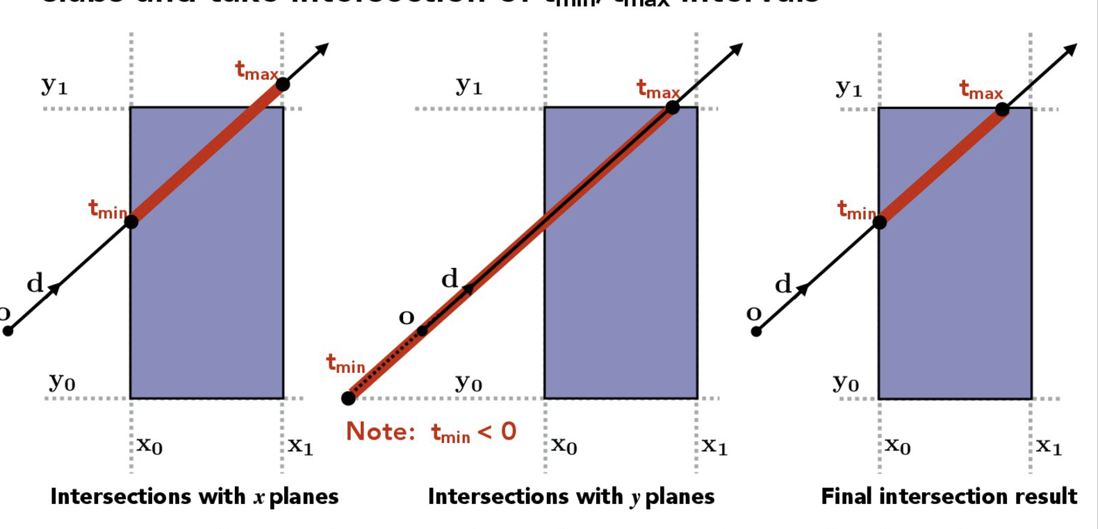
To test if a ray intersects with an axis aligned bounding box, we test if the distances from the origin of the ray to each axis of the bounding box respectively, and find the largest overlapping interval of the intersection segments in all axis. If such an overlapping interval exists, we know the ray intersects with the box. Otherwise, the intersection mises the box. The high level idea in 2D is described below:

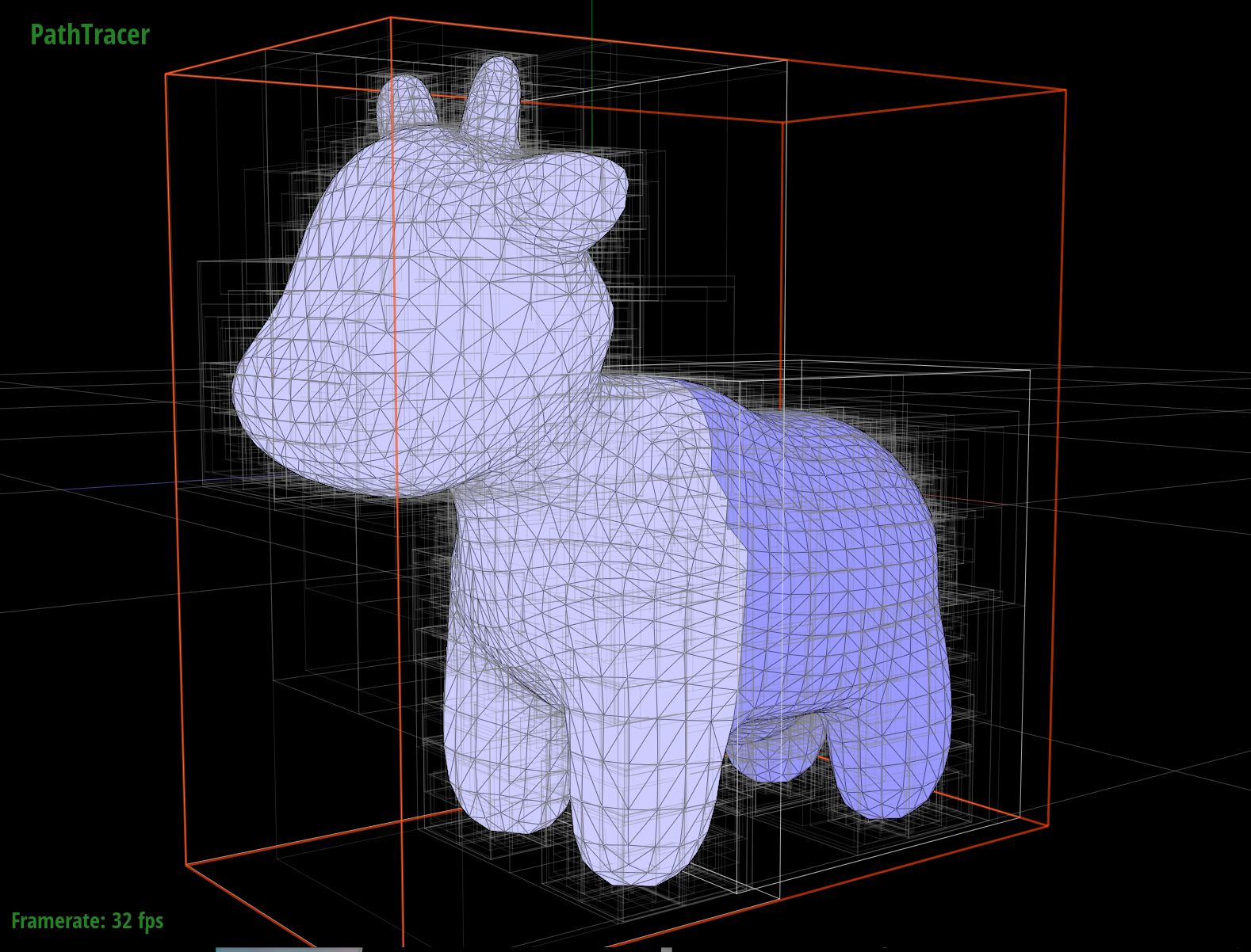
Below is an example of generated bounding boxes around a cow model. As we can see, they do a pretty good job in terms of approximating and bounding the model.

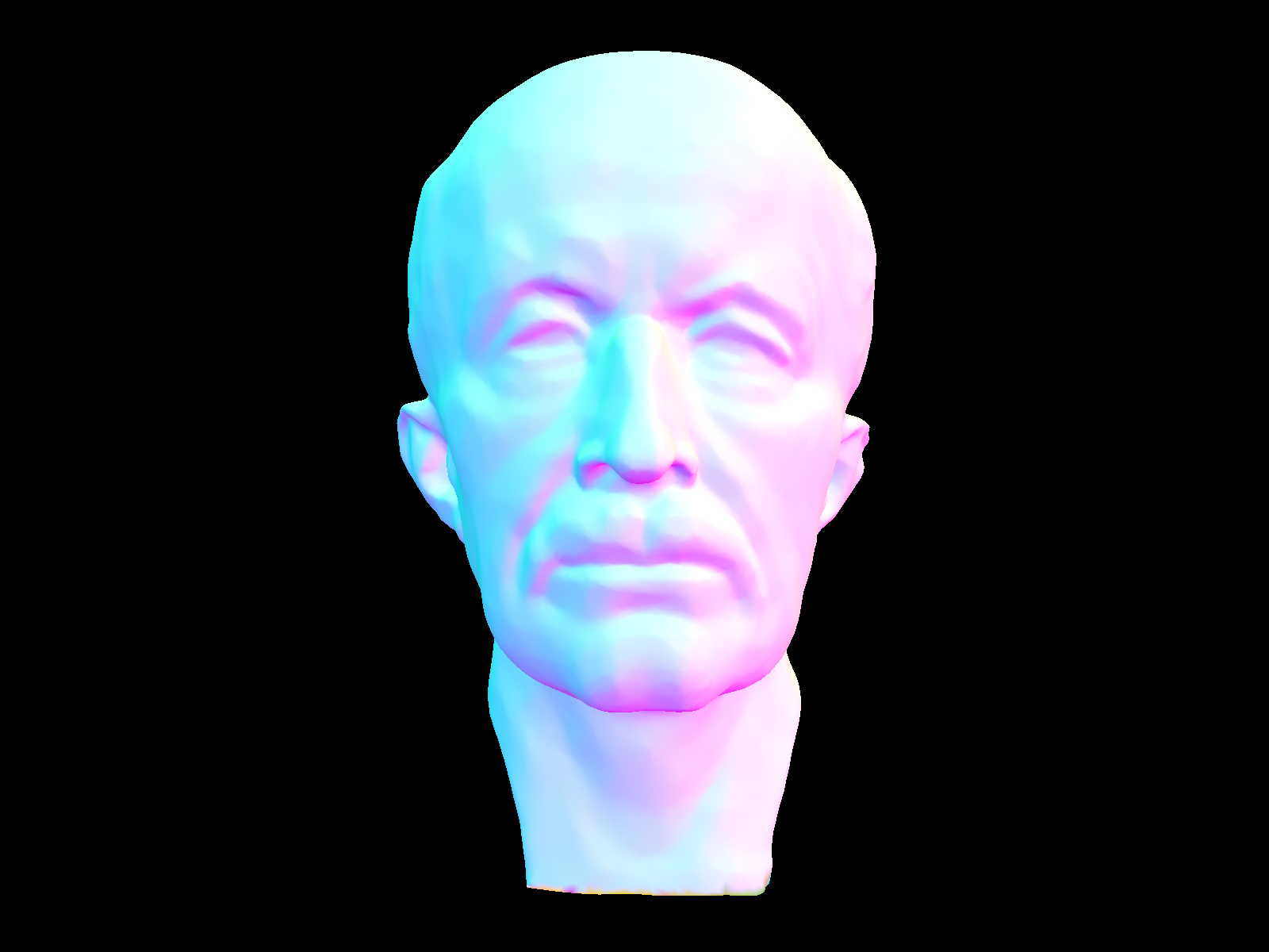
Below are some examples of rendered large .dae files that we usually couldn't render without the acceleration structure:

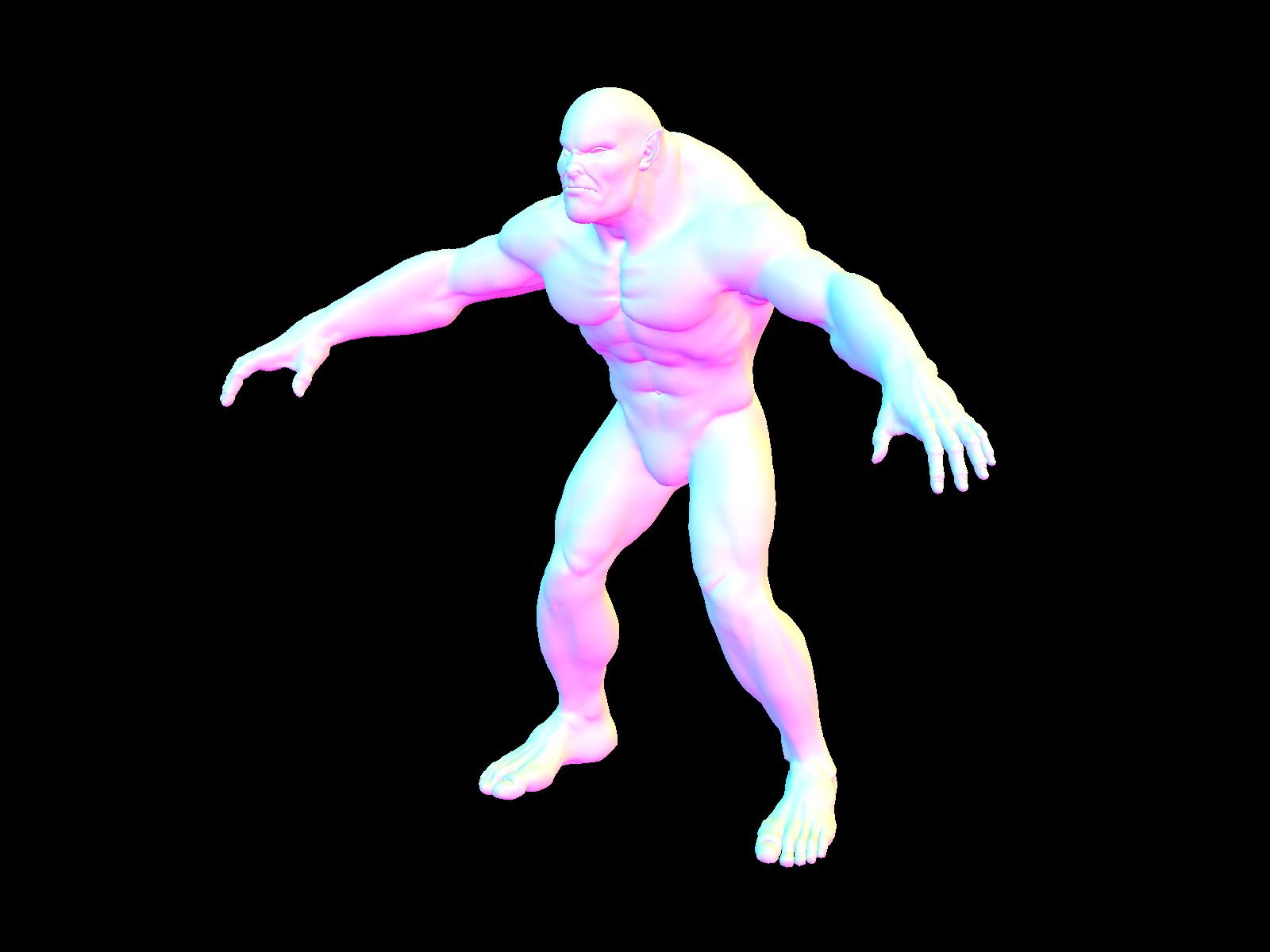
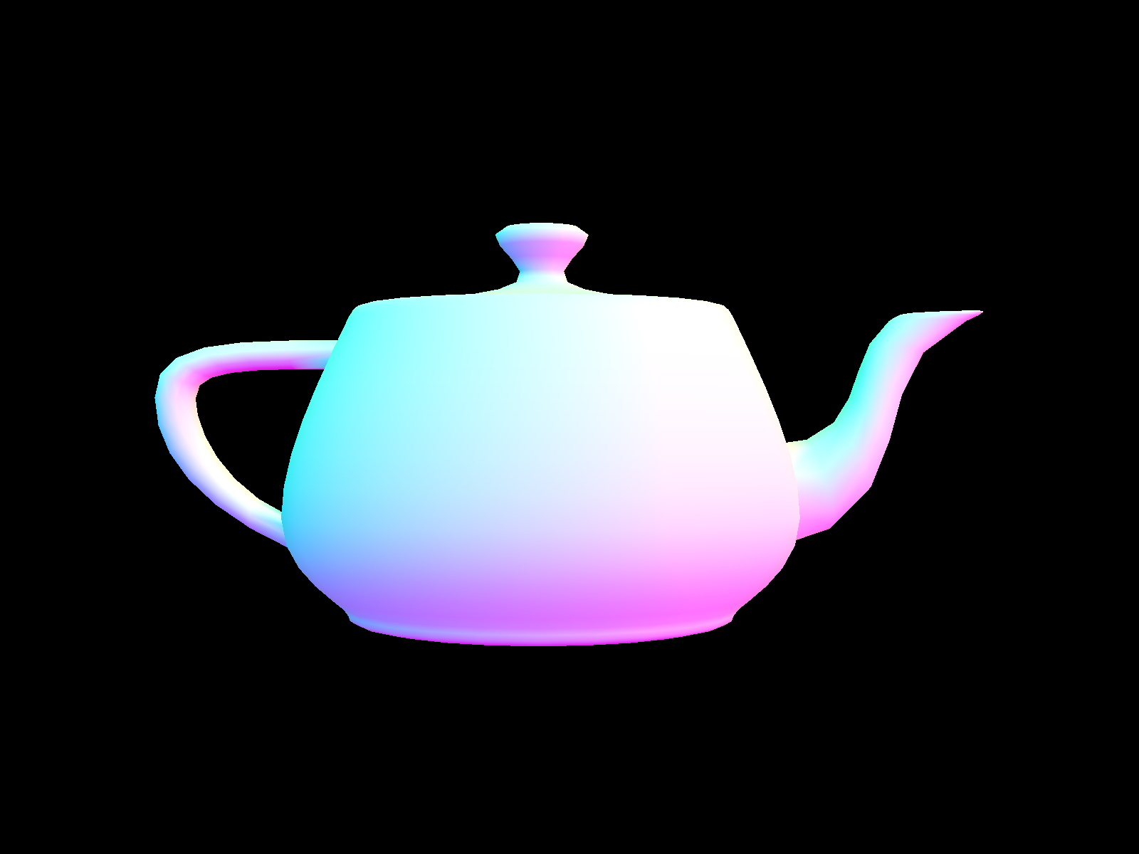
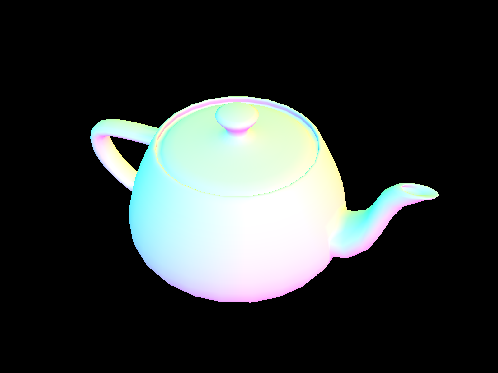
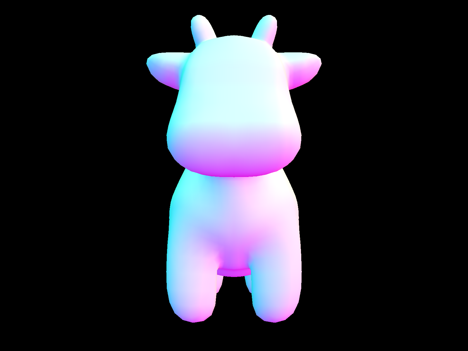
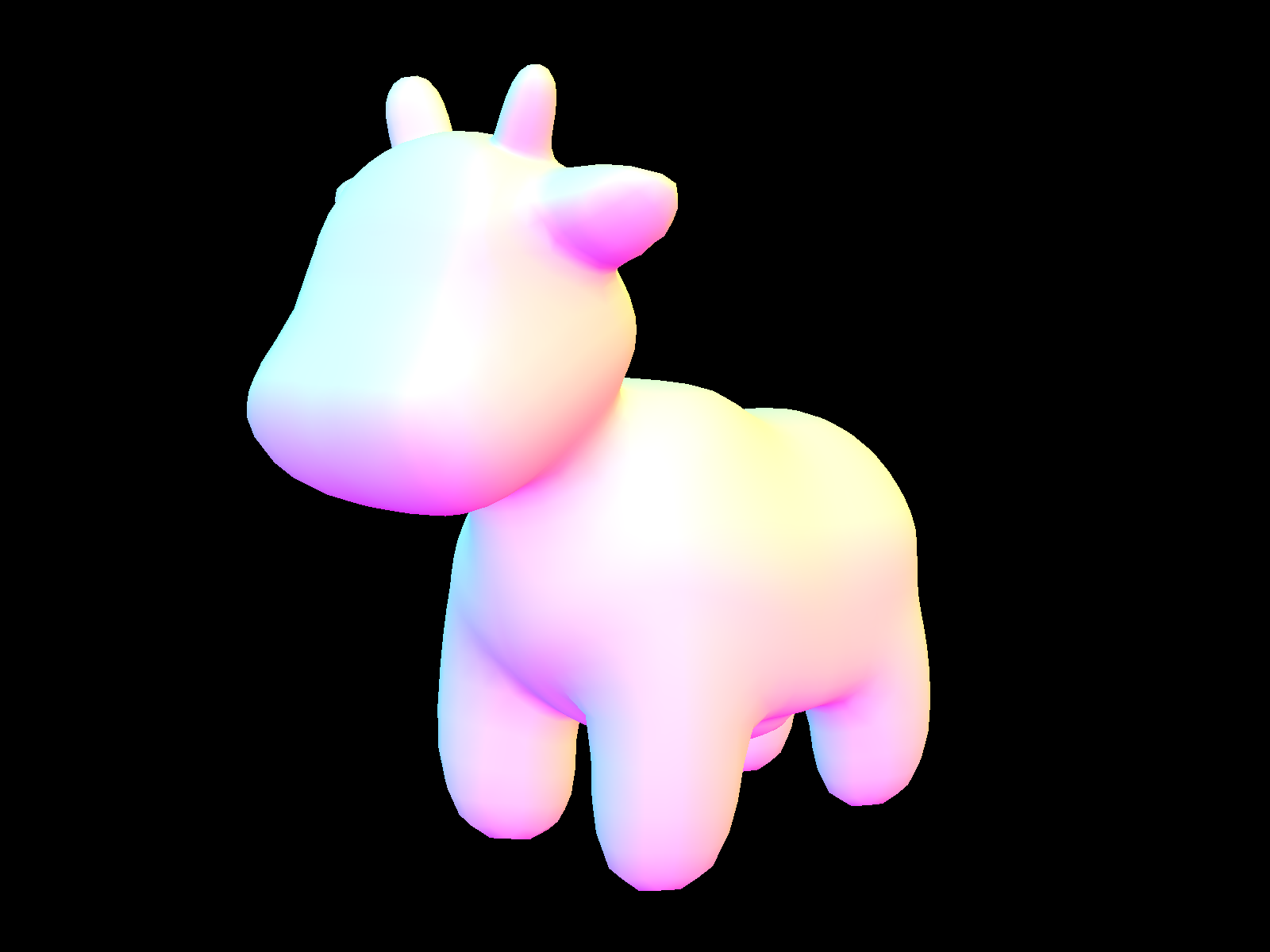
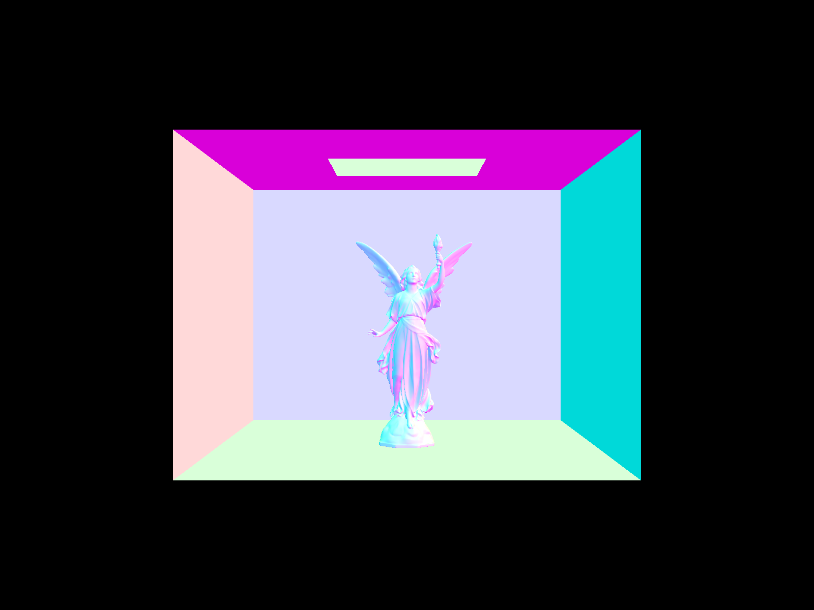
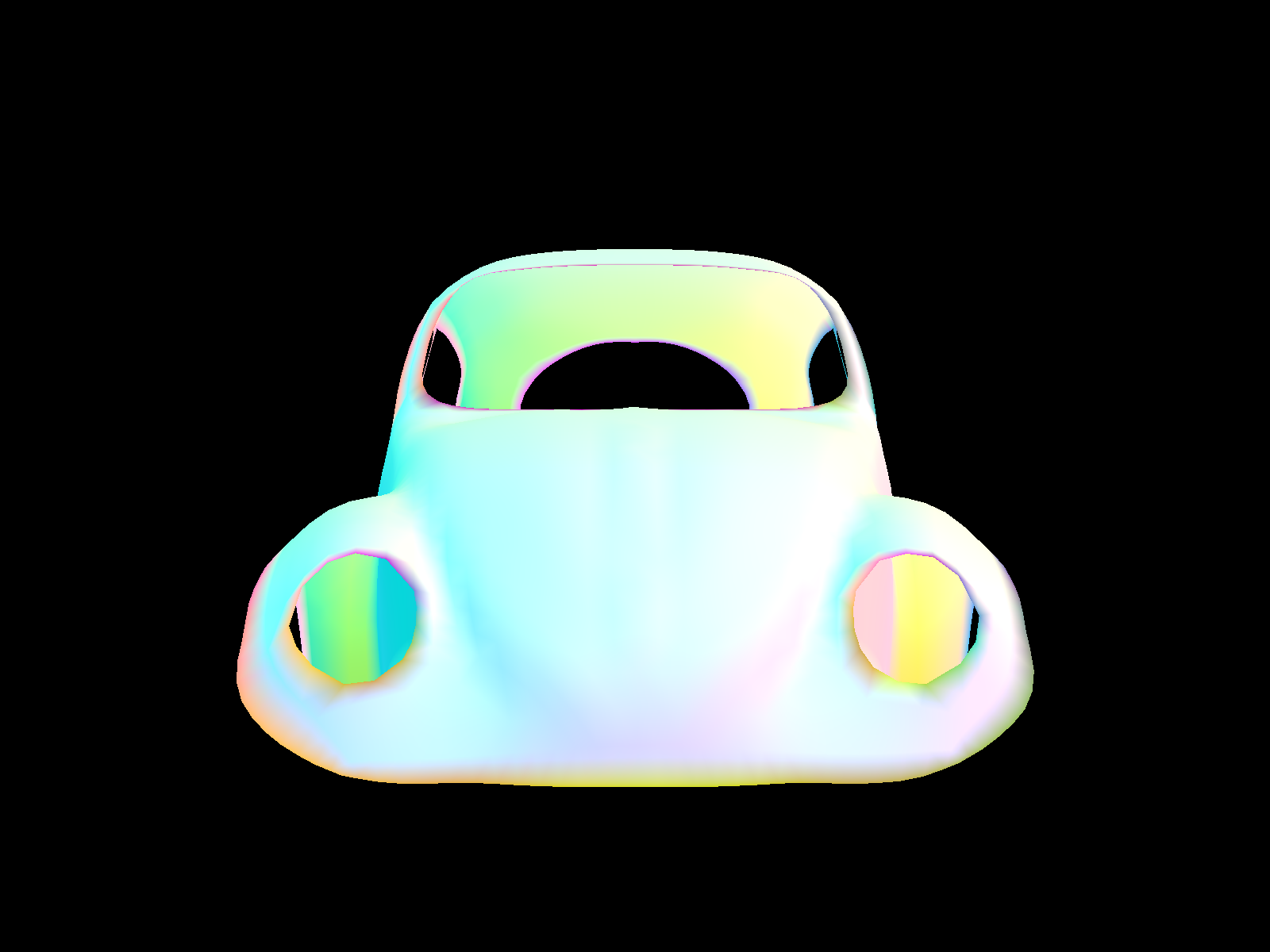
To showcase the effects of the BVH acceleration structure, I conducted the following rendering speed experiments on some of the scenes above.

	Cow	Teapot	Maxplanck	Lucy
Original Rendering Time	938.4110s	394.8520s
Accelerated Rendering Time	2.3335s	1.5884s	2.9929s	1.3188s
Original Avg. Intersection Tests per ray	2958.025862	1215.659140
Accelerated Avg. Intersection Tests per ray	3.154083	2.465466	3.995419	0.971727

As we can clearly see, with the BVH acceleration structure, our algorithm speeds up the rendering time by as much as 469 times! The average number of intersection tests performed on each ray also decreases by a factor of at most 980 times! Specifically, we found that the average of intersections test performed for any particular ray is around 3-4 tests, and the whole rendering time is below 3 seconds. Intuitively, this makes sense. Since our algorithm have partitioned objects into a tree-like structure based on it's spatial information, our intersection algorithm rejects 1/2 of the primitives remaining directly each time if the ray misses the bounding box of either child cluster for all the primitives it contains. As a consequence, we not only have fewer intersection tests with each primitive, reducing the number of computation intensive primitive testing dramatically both per primitive but as a whole. Our intersection algorithm also updates the segment range of a ray when it intersects anything. The intuition behind this is that we are trying to find the closest intersection of a ray amongst all objects, so the intersections beyond an found intersection will never be closer than the current intersection. Thus, the future testing of primitive intersection also gets sped up, resulting in a very small amount of intersection tests performed on each ray.

Part 3: Direct Illumination

In this project I implemented two direct lighting functions. One is uniform hemisphere sampling, and the other one is importance sampling by sampling over lights.

In Uniform Hemisphere Sampling, first we shoot a ray and see if it intersects with the bounding box of all primitives. If not, there's nothing to render from this ray because the ray doesn't bounce off any object. If the ray intersects with any object, we sample a number of directions at the intersection point over hemisphere uniformly in a solid angle. We shot another ray from the intersection point to each of the randomly sampled outgoing direction and get the radiance along this ray. If the ray hits something, we ask for the radiance at that intersection using it's bsdf. We use Monte Carlo integration to approximate the value of the integration, so we divide the radiance by the probability of sampling an ray in that direction (1/2-pi). Since we also need to take into account Lambert's Cosine Law, which gives us a cosine factor depending on the angle at which the ray enters the hemisphere, we will also divide by the cosine of incoming direction. The resulting value will be the irradiance from the environment at that intersection point using uniform hemisphere sampling.

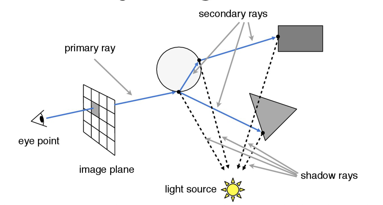
In Importance Sampling Over Sampling Lights, the idea is generally the same as the uniform hemisphere sampling but now we actually know where the lights are so we sample them directly, so we will loop through each scene light. If it's a delta light, we sample only once. Otherwise we still sample multiple times like the uniform hemisphere sampling. We also get value of the pdf, bsdf, and distance to the intersection point directly from a spectrum sampled from the light.

Below is an example of the idea in the realm of ray tracing:

Below we compare the images rendered with both implementations of the direct lighting functions respectively: (1) Uniform Hemisphere Sampling, and (2) Importance sampling by sampling over lights (Lighting Sampling):

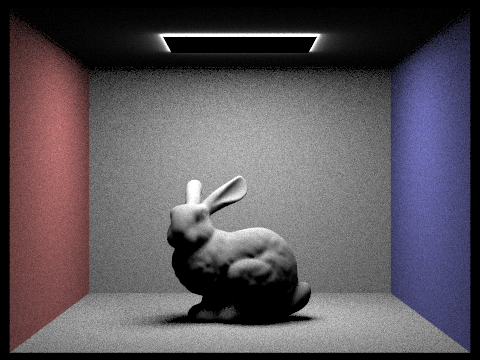
As we can see, there are a few differences between the hemisphere sampling and lighting sampling under same parameters. First, as we can see, the uniform hemisphere sampling produces more noise than the importance sampling. This makes sense because in lighting sampling we actually know where the lights are, so we are making more informed sampling decisions. Second, as we can see from the lighting on the head of the rabbit, the uniform hemisphere sampling seems to produce more light and make the image brighter than the lighting sampling. Overall, it seems that lighting sampling produces better quality results because the lights are more uniformly spread and the noise level is small.

Below we compare the noise levels in soft shadows of the bunny scene (with at least one area light) at various number of light rays, fixed at 1 sample per pixel using lighting sampling:

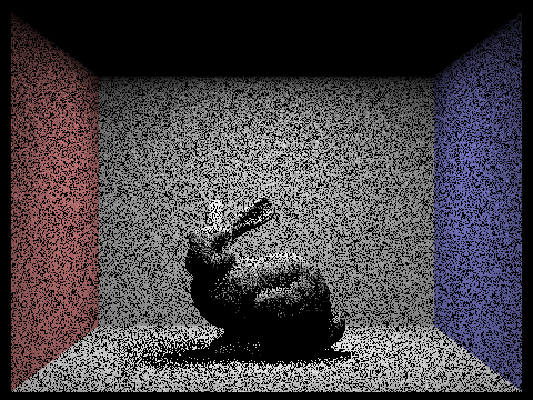
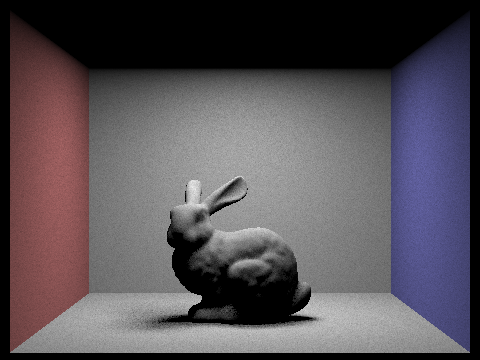
As we can see, with more light rays, the noise level in soft shadows decreases and the image also looks much smoother and relativistic.

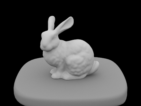
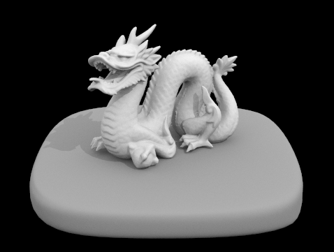
Below I show more rendering images rendered through lighting sampling:

Part 4: Global Illumination

Aside from the direct illumination, we can also render images using a combination of direct and indirect illuminations.

To implement the indirect lighting, I adapt the idea of Russian roulette. In a high level, the idea is that we first calculate the illumination from the ray hitting anything and then bounce the light rays off and keep calculating the radiance and irradiance with a certain probability. However, like a Russian roulette, it has a probability to terminate and not bounce off anymore, or until the manually set limit for the max amount of depth is reached. I implement this by setting the depth of rays initially to the max ray bouncing depth, and recurse on the function to keep calculating the radiance with a probability of 0.6. We multiply the result with the spectrum sampled from the light, multiplies with the cosine term, divide by the pdf from the sampled bsdf and also divide the probability of not terminating the recursion (0.6) to get the actual expected radiance.

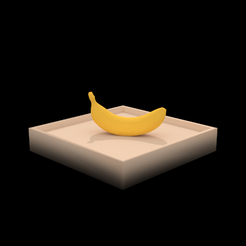
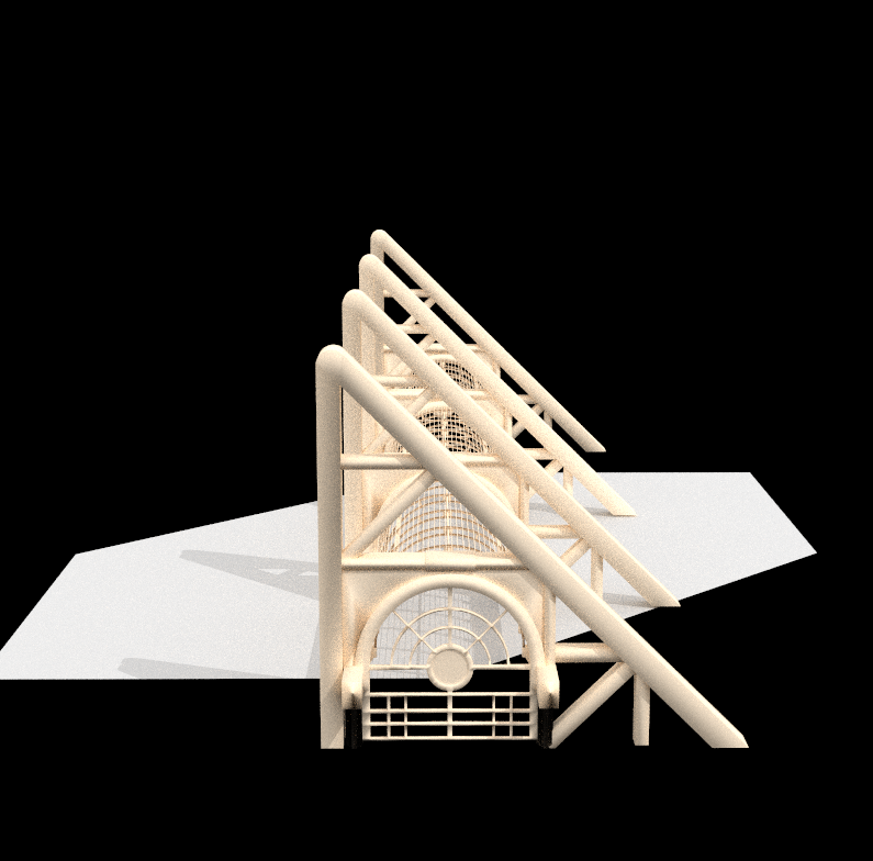
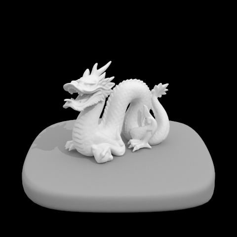
Below are some examples of images rendered with global (direct and indirect) illumination:

Now, we will compare rendered global illumination views with both only direct illumination, then only indirect illumination:

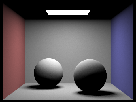
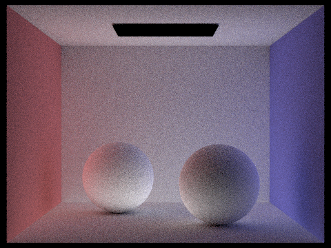
Now, we will compare rendered views with different max_ray_depth (the max number of ray bounces):

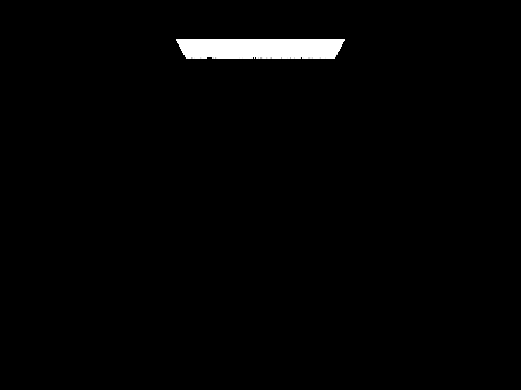
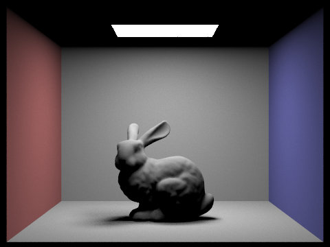
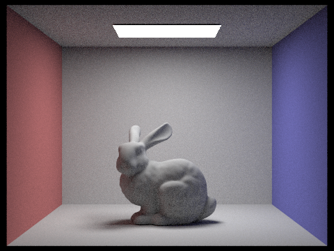
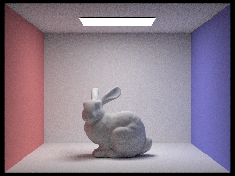
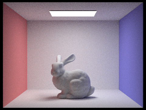
As we can see, with more bounces of light, the images become brighter but converge to a uniform lighting pretty quickly so the rate of illumination boast decreases as we have more bounces of light, and of course, longer time is needed for the rendering.

Now, we'll compare rendered views with various sample-per-pixel rates:

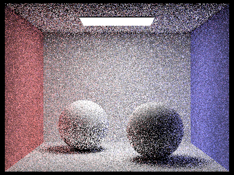
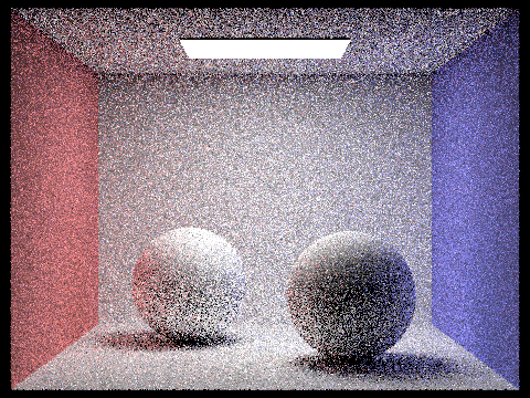
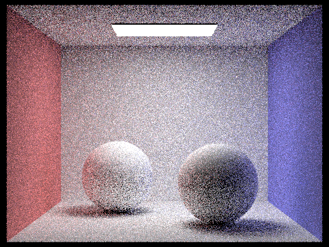
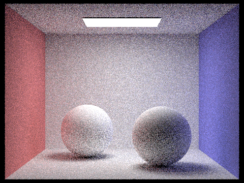
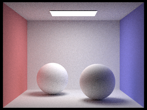
As we can see, the noise level in soft shadows decreases as we have more samples per pixel, and of course, longer time is needed for the rendering. Also, for a sample-per-pixel of 1024, the image looks mostly noise-free at a very high quality.

Part 5: Adaptive Sampling

As we see previously, Monte Carlo path tracing is very powerful in generating realistic images, but it always results in a large amount of noise, which can be eliminated by increasing the number of samples per pixel. The number of computations needed increases linearly with the sample rate.

However, it turns out that we usually don't have to do this uniformly for all pixels. Some pixels converge faster with low sampling rates, while other pixels require many more samples to get rid of noise. Thus, we can adapt statistics to early-stop sampling on certain pixels if we are confident enough that the pixel values have converged.

My adaptive sampling algorithm works like this. For each sample ray we draw, we calculate a spectrum of radiance from that sample ray. We keep a running statistics of the average illuminance and variance so far for the specific pixel we are computing the radiance on, as we draw more sample rays. We stop sampling when we are 95% confident statistically that the pixel has converged, based on the variance and average illuminance for the number of samples drawn so far.

Specifically for the implementation of the adaptive sampling algorithm, I keep two variables: one storing the running sum of illuminance and the other storing the running sum of the squared value of the illuminance. By doing so, we can use a quick formula to calculate the mean and the variance, without storing the illuminance for each sample. Then, instead of checking for a pixel's convergence for each new sample, we want to avoid computing it any more frequently than we need to, so for every samplesPerBatch, we calculate the mean and the variance based on the two variables stored above. Then, we check if I=1.96 * sigma / sqrt(n) where sigma is the standard deviation and n is the number of samples that we have sampled so far. We stop sampling once I < maxTolerance * mu where maxTolerance is a ratio of the margin of error we can accept for statistical confidence and mu is the mean.

Below is an example where we could clearly see the visible sampling rate difference over various regions and pixels in the adaptive sampling method, given the same noise-free rendering

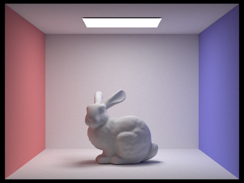
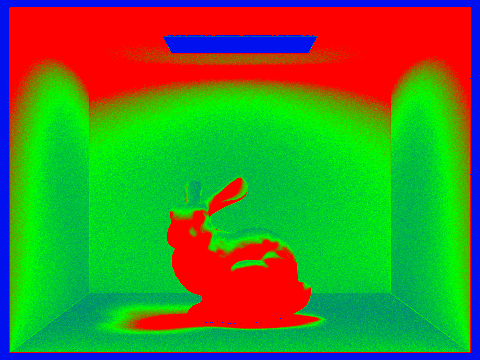
It's clearly visible that the sampling rate is mostly concentrated on the rabbit itself and the ceilings; not much in the light; and medium on the side walls and the floor. The adaptive sampling thus avoids the fixed high number of samples per pixel by concentrating the samples in the more difficult parts of the image, reducing the unnecessary computations and speeding up the rendering.